Hammer-Nørskov, Bhattacharjee-Waghmare-Lee and the $d$-band center model

Hello, hello! Did you think I would never come back? Well, while my Hartree-Fock magnum opus still working in progress, nothing holds me back to write little things about my daily work routine.

So, as a computational chemist dealing with material science, particularly under the catalysis umbrella, I spend a great deal of time translating some sort of math from the gods of science to our human world.

One of those gods that I like is Nørskov, his literature is incredible and I appreciate a lot the simplicity of his thoughts and the power it brings to us chemists. If you ever have worked with heterogeneous catalysis you have faced the d-band theory, which states that the closer the d-band center gets to the Fermi level, the stronger the adsorbate adsorption will be, and the worst it becomes for a catalytic process.

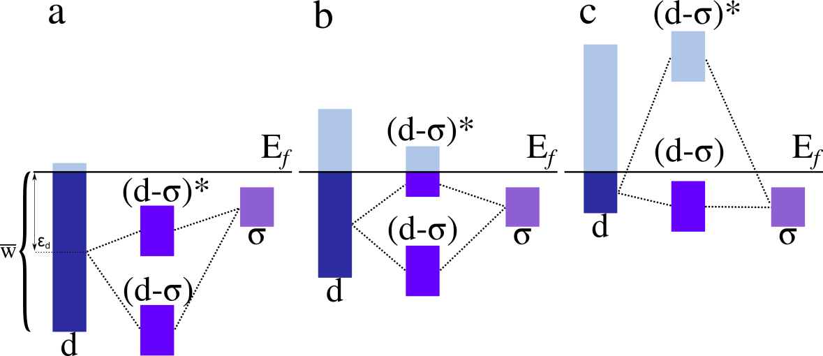
So, to better understand this we may see what is happening through a picture as figure 1. You see, the $\epsilon_d$ corresponds to the d-band center, which goes from a lower value (a) to a greater value closer to the Fermi level (c). The Fermi level is represented by the horizontal black line with a E$_f$ symbol at its end.

Figure 1: d-band coupling with different band centers.

So, as we can see in figure 1a the resultant bands from the coupling of the d-band with the $\sigma$ band from the adsorbate are all filled with electrons. This is, both the bonding ($d-\sigma$) and anti-bonding ($d-\sigma$)$^*$ portions of the band. Therefore, the interaction between the catalyst’s surface and the adsorbate is weak.

On the other hand, as we go to the 1b case we see a slight increase in the $\epsilon_d$, which causes a decrease in the electronic population over the anti-bonding region. Thus, it can be said that the 1b scenario is a slightly better one in terms of bonding interaction strength.

Then it comes 1c, where we have a complete unoccupied anti-bonding band, thus the strongest interaction among the three. So, isn’t that good after all? Well, think about it. You wish to have a working catalyst, isn’t it? So, you may agree with me that if your adsorbate binds too well to the catalyst’s surface it will remain bonded for, well, let’s say: all eternity, MUAHAHAHA!!!

You may be attempted to think that 1a would be our deal, but it came with great surprise that the best answer isn’t that easy. One might be thinking that 1b would then be a good way to go. Well, in fact, that could do it, but be advised that you may take extra precautions.

So, there are a few ways to assess the d-band center of a periodic system. My first love was, for sure, the Hammer-Nørskov method, which is both simple and powerful. However, let’s face it, there are some unspoken problems about how the spin polarization influences the d-band center. Fortunately, there are those three people that came to our rescue: Bhattacharjee-Waghmare-Lee.

The Hammer-Nørskov method allowed us to determine the d-band center as two moments of a density of states plot (DOS). The first moment is simply the average of the DOS, which might be taken as the whole DOS or the electronic occupied portion of the system. I’m not quite sure right now, but I think Nørskov has already pointed out something about the differences it causes to sample the electronic occupied portion and the whole DOS.

The second moment is a simple measure of the bandwidth, which again can be understood in terms of the occupied region or the whole picture of the DOS. For the sake of clarity and from now on, we will concern about the whole DOS. Those expressions can be simply written as equations 1 and 2.

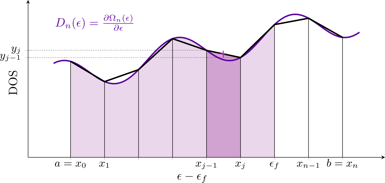
Well, it seems a little scary, don’t you think? Quite honestly speaking the process to solve those equations is quite interesting and easy. Well, there are a lot of strategies one can use. Say you have to do an analysis to an important meeting where you will have to discuss your results, and you have no time to do the best approach of the moment. So, what to do? Well, take some shortcuts. That’s where the trapezoidal rule comes in handy. Let’s take a look at figure 2.

Figure 2: Trapezoidal rule under a portion of a DOS plot.

So, suppose you have used your most beloved quantum chemistry software to compute your super-duper DOS. Now what? Well, you are supposed to extract from it the d-band center, but you look at equation 1 and realized: “crap, how am I supposed to compute an integral on my table of $x$ and $y$ values? Fear not little one, we will do it together.

As you can see, figure 2 represents our DOS and we plotted it based only on our $x$ and $y$ computed values, where the $x$ values were corrected by the Fermi energy. So, to use the trapezoidal rule you might do as proposed by figure 2.

You have to get small portions under the area of the curve that describes your DOS plot, then compute their area and sum them up. Boom! You got it. Well, not so fast. You first need to decide what is the size of the $dx$ value you are going to consider, what about the $dy$ one? Well, if you already have a vector of $x$ values, and another of $y$ values you can simply do 5 easy steps:

1. Compute the product of DOS and energy levels as the product of vectors $x$ and $y$;
2. Take the $\Delta x$ value from the intervals for each pair of points in your $x$ as $x_j - x_{j - 1}$. You shall proceed to the same rationale to the $y$ vector, but this time taking as the sum $y_j + y_{j - 1}$. For both cases you will end up with a vector $n - 1$ elements where $n$ is the number of elements of your starting vector;
3. Sum up the product from step 1 for each pair of points two at a time in a way you get $n-1$ elements;
4. Compute the area for the product of step 1, which will be the numerator of equation 1, and for the $x$ and $y$ intervals of step 2, which will be the denominator of equation 1.
5. Then just sum them up and take their ratio;

So, let’s see how it looks like when using Python. Have you forgotten that my deal is put python elsewhere? MUAHAHAHA! Brace yourself, here it goes:

def first_moment(dpdos, pdos, Ef):
    Edos = pdos - Ef
    e = dpdos * Edos
    dx = array([ey - Edos[idx-1] for idx, ey in enumerate(Edos) if idx > 0])
    dy = array([ey + dpdos[idx-1] for idx, ey in enumerate(dpdos) if idx > 0])
    dxy = array([ey + e[idx-1] for idx, ey in enumerate(e) if idx > 0])
    num = (dx * dxy)/2
    den = (dx * dy)/2
    ne = 0
    for idx, e in enumerate(den):
        if Edos[idx+1] < 0: ne += e 
    return num.sum() / den.sum(), ne

If you pay attention, for our python function we provide the DOS plot we want to evaluate as two separated vectors dpdos and pdos, the first corresponds to the $y$ values and the second to the $x$ values. We also give the Fermi level as $E_f$. Nevertheless, if you look it closely you will see that our function not only returns the d-band center but also the number of electrons for that given DOS. Not bad, eh?

Now, let’s evaluate the second moment from the equation 2. I haven’t said a word about a particular variable present in this equation, the $f_d$, which stands as the fractional occupancy of d-band of the sampled metal. Here things start to get a little blurred because the $f_d$ definition is somehow ill-defined. But, for the sake of clarity, we can understand $f_d$ as the ratio between the electron filling of the d-band and its actual electronic capacity.

So, with the total number of electrons we retrieved from our first-moment evaluation, we can compute the $f_d$ by dividing it by the total number of electrons the d-band of a metal atom can hold, this is, $ne/10$. Hence, we can compute the bandwidth.

def second_moment(fd, dcenter):
    return (1./3.) * (( (1./(0.5-fd)) * dcenter)**2) * (1. - ( 3. * fd ) + ( 3. * fd**2 ))

Great, now we can compute the first and second moments. But, remind yourself that I told you about some problems from the Hammer-Nørskov. Those problems arise when you don’t consider how the spin polarization of the system can affect the d-band center. Thus as a way out of this Bhattacharjee-Waghmare-Lee proposed a fix as shown by equation 3.

Now we can simply use the first moment defined by Hammer-Nørskov to find the d-band center for each spin channel, up ($\uparrow$) and down ($\downarrow$), as well as for the fractional occupancy.

That’s all, folks! I hope you enjoyed it. :)