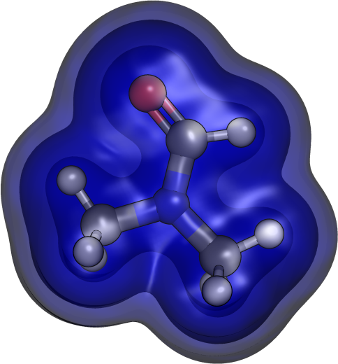
Computing isosurface volume
19 Feb 2021
So my first writing is going to be about something that brought me joy. No, seriously, it did really bring me joy! I’m not kidding. Because, as you may have guessed, I do love python programming language and nothing could bring me more joy than figuring out things from nowhere.
First, be advised that I’m not a professional programmer, neither a computer scientist and most of the things I know now about dealing with computational things related to chemistry I learned by trial-and-error. Therefore, do not expect to find here the state of the art of anything. Now, without further ado let’s dive in.
Suppose you have computed the electronic density of your system $\rho(\tau)$ and exported it using a Gaussian cube file format - currently, you can do it in almost any software out there as Quantum-ESPRESSO, Orca, GAMESS, VASP, Crystal, the list goes on.
As you may have noticed, the density is a function of $\tau$, which represents three dimensions $x$, $y$, and $z$.
Since the gaussian cube file format makes use of the bohr radius unit, a finite representation that encompasses all the electronic density must be sampled in that unit system.
The quality of the sample will be given by the size of the grid that was used to write each voxel of the cube. A voxel can be understood as “a 3D pixel” - please, forgive me lords of CS and gods of CG (and some academics).
All those information are typically stored in the header of the cube files, which can be found as the example below:
The first two lines are just labels, and the third line is the number of atoms and origin position for the given cube file. Yet, the next three represents the number of points in each axis, along with the vector that describes that axis.
Finally, you will be given a table that should have the same number of lines as the number of atoms. For three atoms, as our example, you will see three lines. Each line starts with the atom $Z$ number and its position.
All the remaining data will be printed in a very peculiar order. As a cube comprises three dimensions, one should expect that each slice of the cube will be printed as a 2D matrix.
Indeed, that’s what happens, and roughly speaking that matrix is written as a n$\times$6 table, according to the code below:
for ix in range(NX):
   for iy in range(NY):
      for iz in range(NZ):
         print("{:15.10f} ".format(data[ix][iy][iz])
         if iz % 6 == 5:
            print("\n")
      print("\n")
Therefore, as we are going to compute only the volume of a given isosurface, we are interested in identifying which value of $\rho(\tau)$ is within the isosurface value of our choice.
Once we identified those values, we can sum them up and multiply them to the cubic value of one voxel. However, we need to compute the voxel volume before going on in our quest.
Hence, let’s retrieve the size of each axis, the matrix of the cube lattice and the sum of all the values that are higher than a specified isosurface value.
from numpy import array, sqrt, sum, zeros
points = zeros(3)
M = zeros([3,3])
with open(CUBE, 'r') as cube:
    v = 0
    next(cube)
    next(cube)
    idx = 2
    for line in cube:
        if idx >= 3 and idx <= 5:
            l = line.split()
            points[idx-3] = float(l[0])
            for j in range(3):
                M[idx-3,j] = float(l[j+1])
        if len(line.split()) > 5:
            for val in line.split():
                if float(val) > iso:
                    v += 1
        else: pass
        idx += 1
Once we got those values we can proceed to some computations. For instance, to determine the voxel volume we need to compute the total volume of the cube and divide it by the number of voxels within the cube.
As matrix M, from our code, is the reduced matrix of the cube, we need to get the original matrix back by multiplying it by the number of points of each axis. So, here is the trick:
M = (M.T * points).T
Vm = sqrt(sum(M**2, axis = 1))
voxel = Vm.prod() / points.prod()
Now we can calculate the bohr volume, then convert it to any unit we like. I will present the conversion to Å and cm$^3$/mol.
A2m = 1e-30
Na = 6.02214076e23
m3tocm3 = 1e6
bohr2A = 0.14818474347690475
Vbohr = v * voxel
Va = Vbohr * bohr2A
Vcmmol = ((Va * A2m) * Na) * m3tocm3
Now, we can print the result and get the volume from variables Vbohr, Va, and Vcmmol for bohr$^3$, angstrom$^3$ and cm$^3$/mol, respectively.
Below are some results that I got by using Quantum-ESPRESSO generated cube files for Ar, CO$_2$ and DMF by employing an isosurface value of 0.001 bohr radius.
| Molecule | Å$^3$ | bohr$^3$ | cm$^3$/mol |
|---|---|---|---|
| Ar | 32.41 | 218.69 | 19.52 |
| CO$_2$ | 45.80 | 309.11 | 27.58 |
| DMF | 108.42 | 731.68 | 65.29 |
Sure you can easily plug and play with this code, create your own script that automates the process and make functions out of those routines. I also recommend you to use the package prettytables from python. It is wonderful. :)